Nanite at Home
As modern GPUs evolve to become more capable and flexible, and assets more complex, rendering scenes that can reach a few million triangles can end up doing unnecessary work. In such scenarios, the culprits are mostly:
- Draw call overhead, which can slow down performance by limiting CPU time and therefore the CPU won't be able to feed the GPU fast enough.
- Vertex and attribute fetch for primitives that are not even visible (outside the camera frustum, backfacing, or triangles smaller than pixels).[1]
Draw call overhead can be reduced by batching, which is compacting draw calls that share a pipeline into a buffer that can be sent over to the GPU using a single call.
For the second problem, however, it is a lot less straightforward. Using a traditional rendering pipeline, one of our options is frustum culling. We can check if the bounds (sphere, AABB, OBB etc.) for each object fall inside the camera's frustum. This can filter a significant number of triangles. However, due to the lack of per-mesh granularity, especially for meshes with high triangle counts and/or big bounding volumes, we might hit another bottleneck. Either we render all the triangles in the mesh, or none at all.
Another way to mitigate high triangle counts is to have LODs for each mesh, where we switch to coarser meshes as the camera moves further away from objects. While this is great at reducing triangle counts, if the LODs have too much error due to simplification, the transitions between levels can be very easy to spot. Artists can model these LODs themselves and therefore have more control over the transitions, but this is a very time-consuming (and often gruelling) procedure that they are most likely better off spending their time on something more productive.[2] And once again, this LOD will be picked for the entire mesh, which can make the transitions even more apparent.
These are precisely the problems that Unreal Engine 5's Nanite set out to solve. Nanite is a virtualized geometry system that uses GPU-driven rendering, mesh clustering, and hierarchical LODs to render massive amounts of geometric detail without the traditional bottlenecks.[3] While I won't be replicating Nanite exactly (hence "at home"), the techniques explored here, meshlets, GPU culling, and seamless LOD transitions, form the foundation of such systems.
This post won't be a step-by-step guide, but it's written so you can follow my thought process. The source code for the demo and renderer I've put together in ~8 weeks can be found at github.com/knnyism/Kynetic.
For my implementation, I decided to use Vulkan as the graphics API and slang as the shading language. To generate my meshlets (or clusters), I've used meshoptimizer and its companion library clusterlod.h.
Setting up the renderer
Before diving into GPU-driven techniques, I wanted to establish a baseline with a traditional CPU-driven rendering pipeline. This gave me something concrete to compare against when it came to analyzing the benefits of GPU-driven rendering.
The CPU-driven pipeline supports merged mesh buffers, instancing and frustum culling. It is set up in a way that we can transition to GPU-driven smoothly.
Merged mesh buffers
A common bottleneck in rendering many meshes is the overhead of binding different vertex and index buffers for each draw call. Even with modern APIs like Vulkan, switching buffers has a cost. One thing that we can do is going "bindless". When bindless is mentioned, it basically means we only bind our buffers once before we make our draw calls, instead of binding them per-call.
Instead of each mesh owning its own GPU buffers, we allocate one large buffer for all indices, one for all positions, and one for all vertex attributes. Each mesh then stores an offset into these merged buffers rather than owning the buffer itself.
I chose to keep positions separate from other vertex attributes. Positions are accessed much more frequently during vertex processing (transforms, culling), while attributes like normals and UVs are only needed during shading. Keeping them separate can improve cache efficiency.[4]
void
With this setup, we can bind the merged index buffer once and use firstIndex and vertexOffset in our draw calls to select the appropriate mesh data. This is a prerequisite for both efficient instancing and indirect drawing.
In my implementation, I made extensive use of VK_KHR_buffer_device_address and push constants. This extension allows the application to query 64-bit GPU virtual addresses and these addresses have full capability to perform pointer arithmetic.
DrawPushConstants push_constants;
push_constants.instances = scene.;
push_constants.positions = resources.;
push_constants.vertices = resources.;
ctx.dcb.;
ctx.dcb.;
Draw call batching
With merged buffers in place, we can now batch draw calls. The goal is to combine multiple instances of the same mesh into a single draw call using hardware instancing.
The key insight is that we need to process meshes in order, all instances of mesh A, then all instances of mesh B, and so on. I use flecs as my ECS, which provides a convenient way to sort query results:
The comparator sorts by the mesh pointer address. The exact ordering doesn't matter, what matters is that identical meshes are grouped together.
m_mesh_query = m_scene.
.
.
.
.;
With sorted iteration, building instanced draw calls becomes straightforward:
Mesh* last_mesh = nullptr;
m_mesh_query.;
This turns N draw calls for the same mesh into a single instanced draw call, dramatically reducing CPU overhead when rendering many copies of the same object.
for ctx.dcb.;
In the vertex shader, we can use SV_VulkanInstanceID to index into our instance buffer and fetch the correct transform for each instance. To access our vertices with the correct offset, SV_VulkanVertexID can be used:
VertexStageOutput
Frustum culling
Pixel shading is usually the GPU's bottleneck, so the hardware aggressively culls triangles that won't contribute to the final image (those outside the frustum, backfacing, or too small to rasterize). This culling happens in fixed-function units like the Primitive Assembler. But when pixel work is light (shadow maps, z-prepass), these stages can become the new bottleneck.
In order to avoid these bottlenecks, we can perform some coarse culling on the CPU before submitting geometry. Frustum culling is one way to do it, which filters out objects that fall outside the camera's view, preventing the GPU from ever having to process their triangles.
In my implementation, I used a function to extract the frustum planes from the view-projection matrix.[5]
static void
Then for each instance, we can test the planes against the bounding sphere:
The
is_visiblefunction only tests against 4 of the 6 frustum planes (left, right, top, bottom), skipping near and far. This is because objects are far more likely to leave the screen horizontally or vertically than to suddenly move past the near or far plane. For games with a large far plane value, testing against it rarely culls anything useful.
static bool
Now, we can simply wrap the instance addition in a visibility check:
I've noticed that most implementations assume the transform has uniform scaling, so just using the length of one of the rows is sufficient. For the sake of functionality, I decided to support non-uniform scaling which involves getting the maximum from the lengths of rows. If non-uniform scaling isn't something you'd want to support in your engine, do:
scale = length(vec3(transform[0]))
Mesh* last_mesh = nullptr;
m_mesh_query.;
Objects outside the frustum are never added to the instance buffer, so they're never drawn.
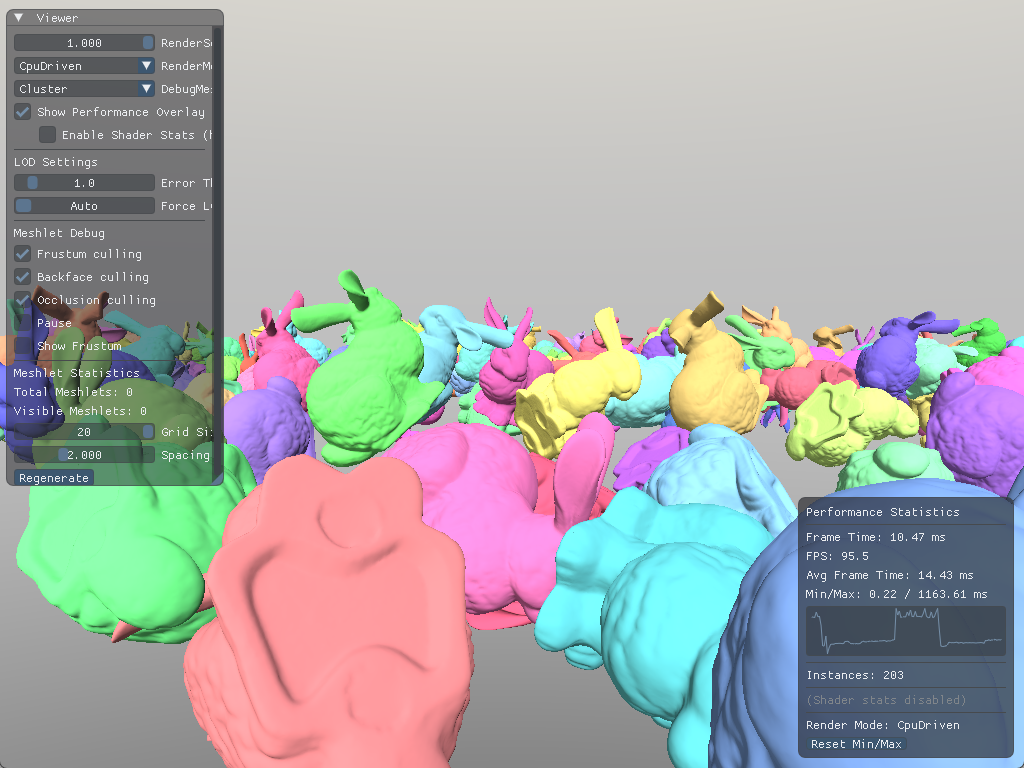
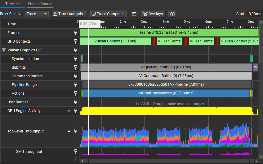
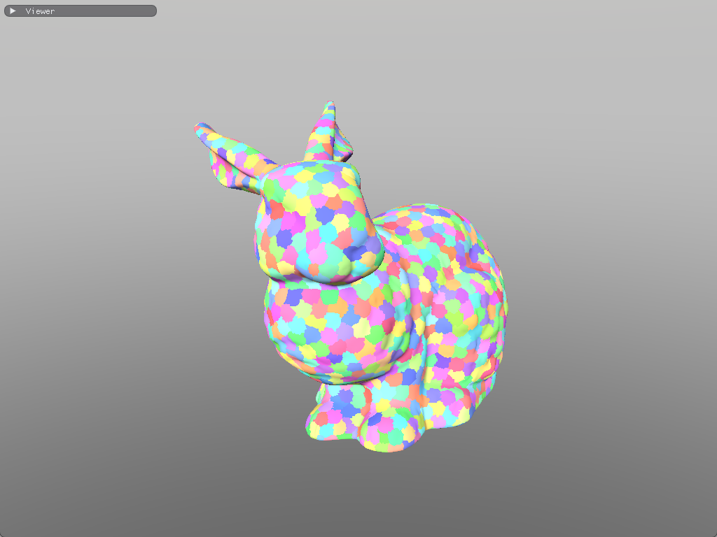
Example scene with 400 bunnies on a grid.

With this very simple visibility check, in this scene, with the camera view shown in the figure, time taken by vkCmdDrawIndexed went from 12.52ms to 7.80ms.
Profiling results
However, once we increase the instance count, and profile on the CPU, the issue becomes clear. We are spending 7.1% of our frame time calculating the bounding sphere in world space and doing the visibility check.

GPU-driven rendering
The CPU-driven approach works and frustum culling filters out objects before they're submitted. However, for scenes with many objects, the CPU still spends considerable time iterating over objects, building instance data, and issuing draw calls, all while the GPU may be sitting idle waiting for work.
The motivation for GPU-driven rendering is to move as much of this work onto the GPU, where it can be parallelized across thousands of threads. The CPU's role shifts from "deciding what to draw" to "uploading all potential work and letting the GPU figure it out."
Multi-draw indirect
The CPU-driven pipeline requires the CPU to issue individual draw calls:
for ctx.dcb.;
Each of these draw calls has overhead. The driver must validate state and translate commands for the GPU. NVIDIA measured ~25,000 draw calls per second at 100% CPU utilization on a 1 GHz processor; at 60 fps, that's only ~400 draws per frame before becoming CPU-bound.[6] Modern CPUs are way faster nowadays, and modern graphics APIs handle draw calls much more efficiently, but the principle still applies.
Vulkan 1.2 introduced vkCmdDrawIndexedIndirect, which reads draw parameters from a GPU buffer. The buffer contains an array of VkDrawIndexedIndirectCommand structs, the same parameters we'd pass to individual draw calls:
;
The buffer needs VK_BUFFER_USAGE_INDIRECT_BUFFER_BIT so it can be used as a source for indirect draws, and VK_BUFFER_USAGE_SHADER_DEVICE_ADDRESS_BIT so the compute shader can modify it later:
void
Instead of the loop, we can just issue a single command:
The engine has a thin wrapper for command buffers, as seen with other code snippets. This function basically maps to
vkCmdDrawIndexedIndirect(cmd, buffer, offset, drawCount, stride).
ctx.dcb.;
With draw commands now stored in a GPU buffer, we've laid the groundwork for something more powerful, which is letting the GPU modify those commands before rendering. Rather than having the CPU iterate over instances and filter them one by one, we can dispatch a compute shader that processes all instances in parallel, writing only the visible ones to the output buffer and updating the draw commands accordingly.
GPU frustum culling
The CPU-side setup changes slightly; instead of culling immediately, we upload all instances and initialize draw commands with instanceCount = 0. The GPU will increment this value within the compute shader for each visible instance.
uint32_t draw_id = 0;
Mesh* last_mesh = nullptr;
m_mesh_query.;
The GPU will receive the instance buffer containing every potentially visible instance, and write to a secondary buffer that contains only the visible instances. This is how I've set it up in my implementation:
void
The compute shader examines each instance in parallel. For visible instances, it atomically claims a slot in the output buffer and copies the instance data:
is_visibleis omitted in the snippet, it's the same logic as the C++ implementation.
FrustumCullPushConstants constants;
void
And the dispatch and synchronization on the CPU side:
FrustumCullPushConstants push_constants;
push_constants.draw_commands = m_draw_buffer_address;
push_constants.instances_in = m_instances_buffer_address;
push_constants.instances_out = m_instances_output_buffer_address;
push_constants.instance_count = static_cast<uint32_t>;
ctx.dcb.;
const uint32_t dispatch_x = / 64;
ctx.dcb.;
// We don't want the GPU to start drawing while we're writing into it
ctx.dcb.;
Finally, we render using the culled results:
While draws with
instanceCount = 0don't rasterize anything, the GPU's command processor still has to parse and skip each one, so there is some overhead. VK_KHR_draw_indirect_count is the same as a normal draw indirect call, but “drawCount” is grabbed from another buffer. This makes it possible to let the GPU decide how many indirect draw commands to execute, which makes it possible to remove culled draws easily so that there is no wasted work.[7]
push_constants.instances = scene.; // Use the output buffer instead
ctx.dcb.;
ctx.dcb.;
Now we can do frustum culling in under 0.03ms:
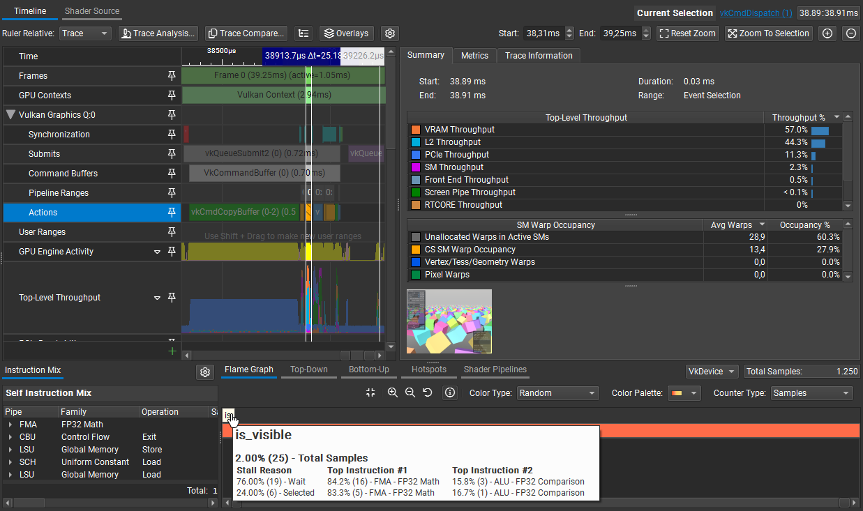
At this point, draw call overhead is (mostly) solved and culling is bringing the draw call count down. The CPU uploads all potential work once, and the GPU filters it in parallel.
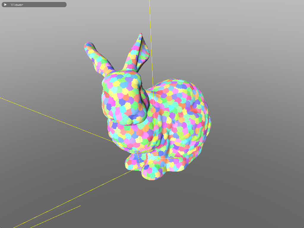
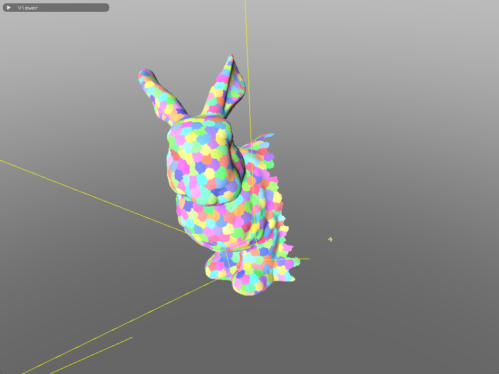
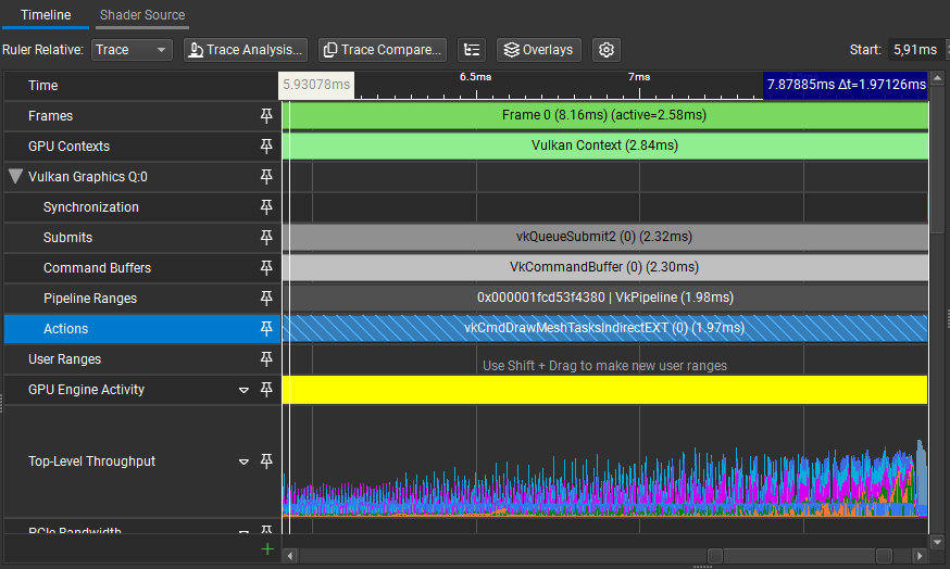
However, we're still processing every triangle in every visible mesh. So, for scenes with high triangle counts, such as this one:
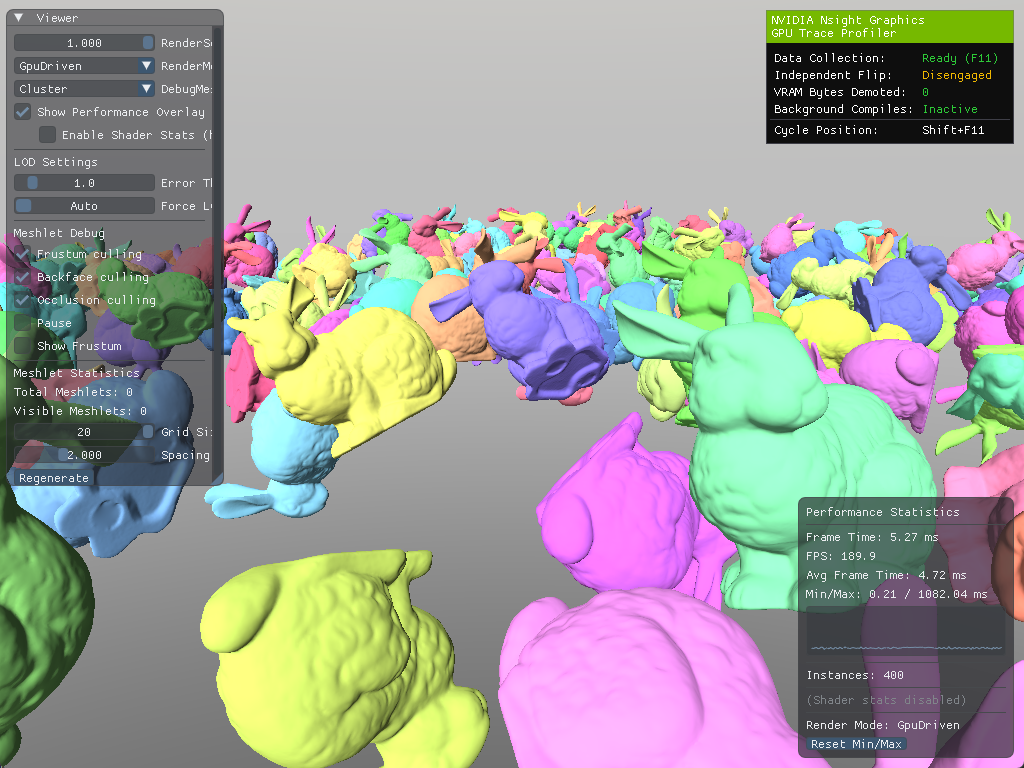
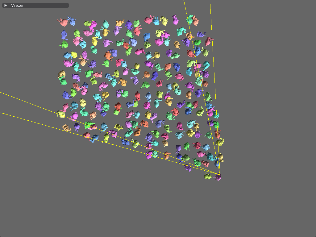
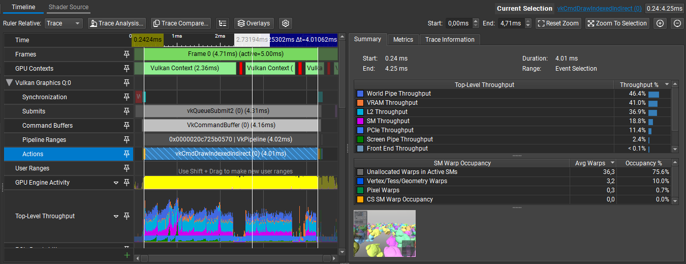
Example scene with 400 bunnies on a grid... Again!
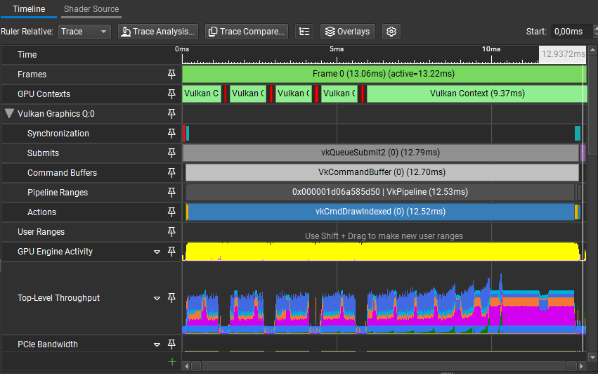
Nsight reports vkCmdDrawIndexedIndirect is taking 4.01ms to draw our bunnies:
The traditional vertex pipeline processes vertices one at a time through a fixed sequence. While this works fine for meshes with small triangle counts, even with culling methods, it does not handle meshes with many triangles efficiently. Each vertex invocation is independent, which makes it difficult to share work or make collective decisions about groups of primitives. Our culling decisions happen either per-object or per-primitive, nothing in between.

Logically, the next step would be to gain finer-grained control over which triangles get processed. Instead of culling entire meshes, we want to cull smaller groups of triangles independently.
Mesh shaders and meshlets
Mesh shaders were introduced to Microsoft DirectX® 12 in 2019 and to Vulkan as the VK_EXT_mesh_shader extension in 2022. Mesh shaders introduce a new, compute-like geometry pipeline that enables developers to directly send batches of vertices and primitives to the rasterizer. These batches are often referred to as meshlets and consist of a small number of vertices and a list of triangles, which reference the vertices.[8]

Mesh shaders reintroduce the pre-rasterization process with two programmable compute-like stages called Mesh and, optionally, Task shaders.
Mesh shaders
Mesh shaders replace vertex and primitive assembly. Each workgroup processes a small batch of vertices and primitives, outputting them directly to the rasterizer. Instead of writing to buffers, mesh shaders emit vertices and primitives through special output arrays.
void
The programming model differs from vertex shaders in a way that, instead of processing one thread per-vertex, we think of it as one workgroup per-meshlet; where threads cooperate to transform all vertices and emit all triangles. In my implementation, each thread handles one vertex and one triangle:
;
if
if
Now that we have an idea of how mesh shaders work, let's look into feeding them meshlets.
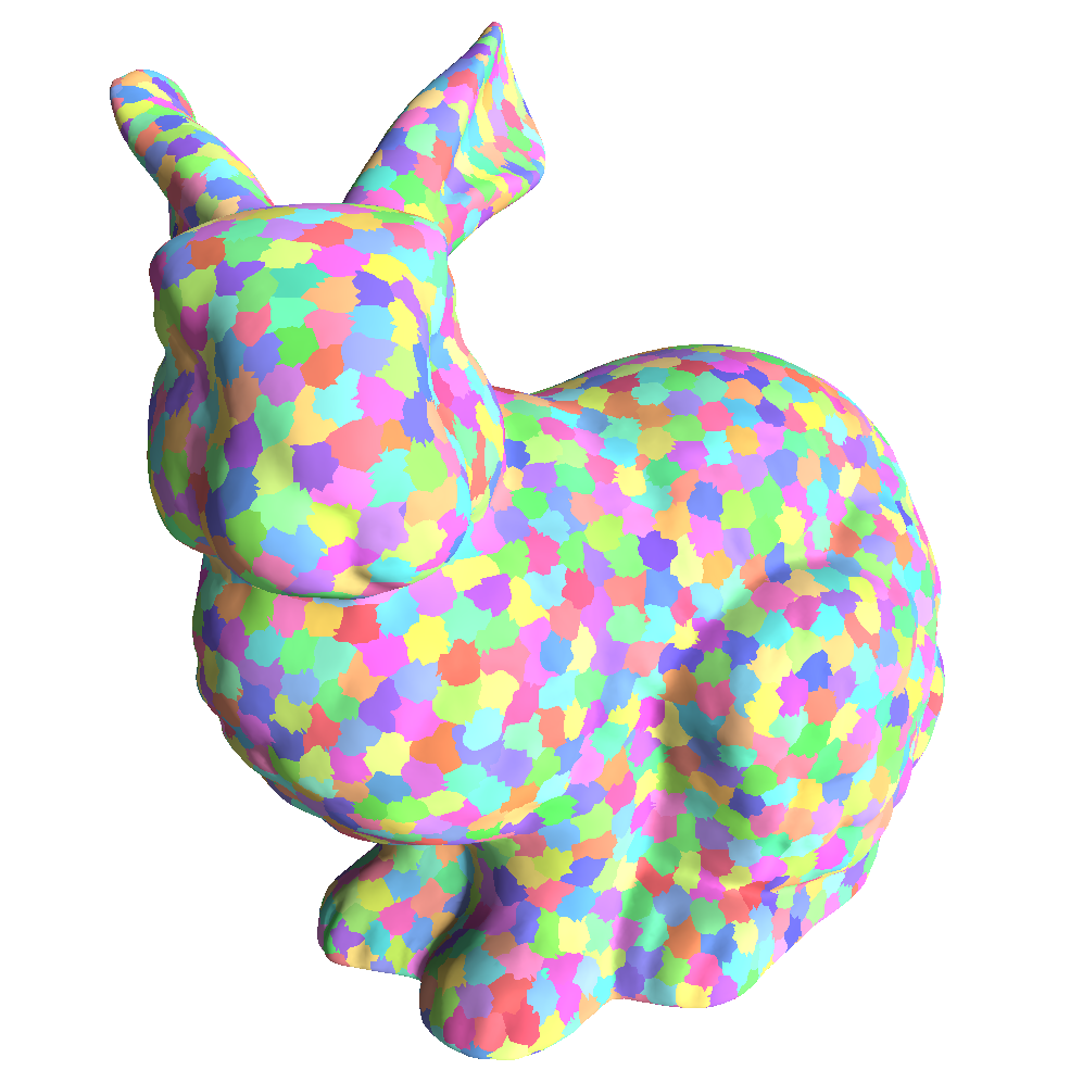
Generating meshlets
The motivation behind meshlets is that most meshes are too large to process efficiently as single units, and processing individual triangles negates our gains from culling. Meshlets find a good balance; small enough for fine-grained culling and large enough for efficient GPU processing.
A meshlet is a small cluster of triangles that share vertices and is large enough to fit in a single mesh shader workgroup. The clusters are generated spatially-aware where adjacent triangles are fitted in a cluster the best way possible. The generation involves maximizing culling efficiency and vertex re-use to reduce bandwidth[9].
For vertex count and triangle count, NVIDIA states:
We recommend using up to 64 vertices and 126 primitives. The "6" in 126 is not a typo. The first generation hardware allocates primitive indices in 128 byte granularity and needs to reserve 4 bytes for the primitive count. Therefore
3 * 126 + 4maximizes the fit into a3 * 128 = 384bytes block. Going beyond 126 triangles would allocate the next 128 bytes. 84 and 40 are other maxima that work well for triangles.[10]— Kubisch, C. (2023)
AMD offers an alternative:
Thus, we suggest to generate meshlets of size
V=128andT=256, as this strikes a good balance between overall performance and vertex duplication. TheV=64andT=126configuration recommended by Christoph Kubisch yields similar performance at the expense of duplicating more vertices.[11]— Oberberger, M., Kuth, B., & Meyer, Q. (2024)
In my implementation, I use EXT_mesh_shader. I've tried both configurations and both of them seem to be performing similarly. So, to favor culling efficiency, I went with NVIDIA's suggestion, which has a lower triangle count per meshlet.
To generate my meshlets, I went with meshoptimizer. meshoptimizer handles meshlet generation with vertex re-use and spatial locality taken into account, we'll just have to make a few calls and populate the data that will be used for our GPU meshlet buffers:
An alternative library you can use is meshlete, however, at the time of writing, the project doesn't seem active.
The
cone_weightparameter controls how much the algorithm prioritizes grouping triangles that face similar directions (useful for backface cone culling). Setting it to0.0fprioritizes spatial locality and vertex re-use instead. We'll revisit this when implementing cone culling.
const size_t max_vertices = 64;
const size_t max_triangles = 126;
const float cone_weight = 0.0f;
// The meshopt_buildMeshletsBound function gives us an upper bound on how many meshlets we'll
// need, which we use to pre-allocate our output arrays. The actual number of meshlets generated
// is typically lower.
const size_t max_meshlets = ;
std::vector<meshopt_Meshlet> meshlets; // vertex count, triangle count, and offsets into
// the other two arrays
std::vector<uint32_t> meshlet_vertex_indices; // maps local vertex indices (0 to vertex_count - 1)
// to the original mesh's vertex indices
std::vector<uint8_t> meshlet_triangles; // triangle indices as uint8_t, where each value is
// a local index into the meshlet's vertex list
meshlets.;
meshlet_vertex_indices.;
meshlet_triangles.;
m_meshlet_count = ;
With meshlets generated, we need bounding volumes for culling. Each meshlet gets two types of bounds, bounding spheres and backface cones. Bounding spheres can be used for frustum culling the same way we were culling instances earlier. Backface cones are going to be used for a different kind of culling which we will revisit later:
;
std::vector<MeshletData> meshlets_data;
for
The buffer setup mirrors what we did for instances; create a storage buffer, copy the data, and pass the address via push constants.
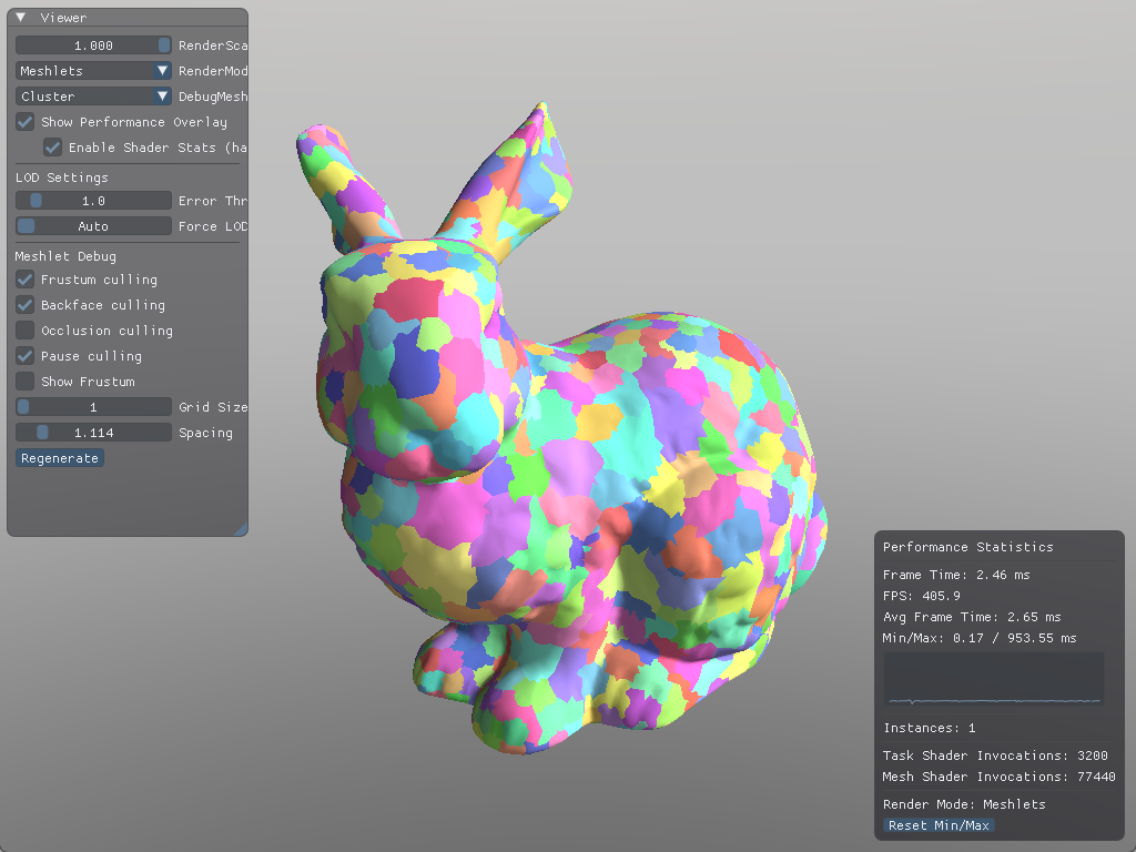
Rendering meshlets
With meshlets generated and uploaded to the GPU, we can now render them using mesh shaders. The key difference from traditional rendering is that we dispatch workgroups rather than draw calls, one workgroup processes one meshlet.
The mesh shader receives the meshlet index via SV_GroupID. Each thread in the workgroup processes vertices and triangles. With our meshlet configuration of 64 vertices and 126 triangles, a workgroup size of 128 threads ensures we have enough threads to handle both:
void
The SetMeshOutputCounts call tells the GPU how many vertices and primitives this workgroup will emit. Unlike vertex shaders where output count is implicit, mesh shaders must declare their output size upfront.
Each thread handles one vertex and one triangle. The work done is very similar to a traditional vertex shader, but indexed through the meshlet's local vertex list:
if
On the CPU side, dispatching meshlets is straightforward. Instead of issuing draw calls, we use vkCmdDrawMeshTasksEXT:
For simplicity, I'm using direct dispatch here rather than
vkCmdDrawMeshTasksIndirectEXT. The indirect variant works the same way asvkCmdDrawIndexedIndirect, dispatch parameters come from a GPU buffer instead of CPU arguments. This becomes useful when a compute pass determines how many workgroups to launch, but for now, direct dispatch keeps things clear.
MeshDrawPushConstants ;
push_constants.positions = mesh->;
push_constants.vertices = mesh->;
push_constants.meshlets = mesh->;
push_constants.meshlet_vertices = mesh->;
push_constants.meshlet_triangles = mesh->;
push_constants.meshlet_count = static_cast<uint32_t>;
ctx.dcb.;
// Dispatch one workgroup per meshlet
ctx.dcb.;
This gives us per-meshlet granularity, but we're still dispatching every meshlet regardless of visibility. The mesh shader runs for all meshlets, even those that are entirely outside the frustum or backfacing.
Task shaders
Task (also called amplification) shaders run before mesh shaders and act as a filter. They examine meshlets in batches, perform culling, and only dispatch mesh shader workgroups for visible meshlets. This is conceptually similar to how our compute shader filtered instances for indirect drawing, but integrated directly into the mesh shader pipeline.
The task shader operates on groups of meshlets. In my implementation, each task shader workgroup processes 32 meshlets:
;
groupshared MeshPayload payload;
groupshared uint accepted_count;
void
Each thread evaluates one meshlet's visibility using its bounding sphere, the same frustum culling logic we used for instances. When a meshlet passes the visibility test, the thread atomically claims a slot in a shared payload and stores its meshlet index:
if
;
After all threads have completed their visibility tests, thread 0 dispatches mesh shader workgroups only for the accepted meshlets:
if ;
Instead of spawning a fixed number of mesh shader workgroups, using DispatchMesh, we can spawn exactly as many as we need. Culled meshlets never invoke the mesh shader at all, saving significant work compared to culling inside the mesh shader itself.
On the CPU side, we dispatch task shader workgroups instead of mesh shader workgroups directly. Since each task shader workgroup handles 32 meshlets, we need to make a small adjustment:
uint32_t task_count = / 32;
ctx.dcb.;
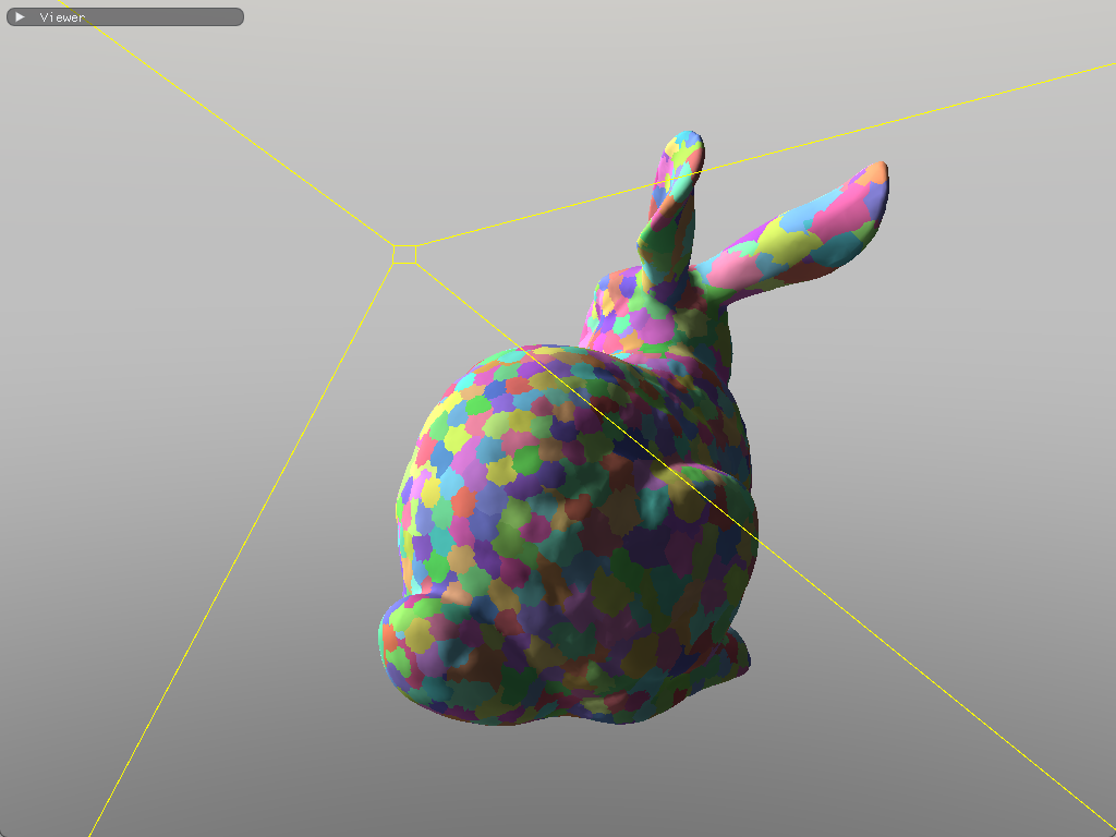
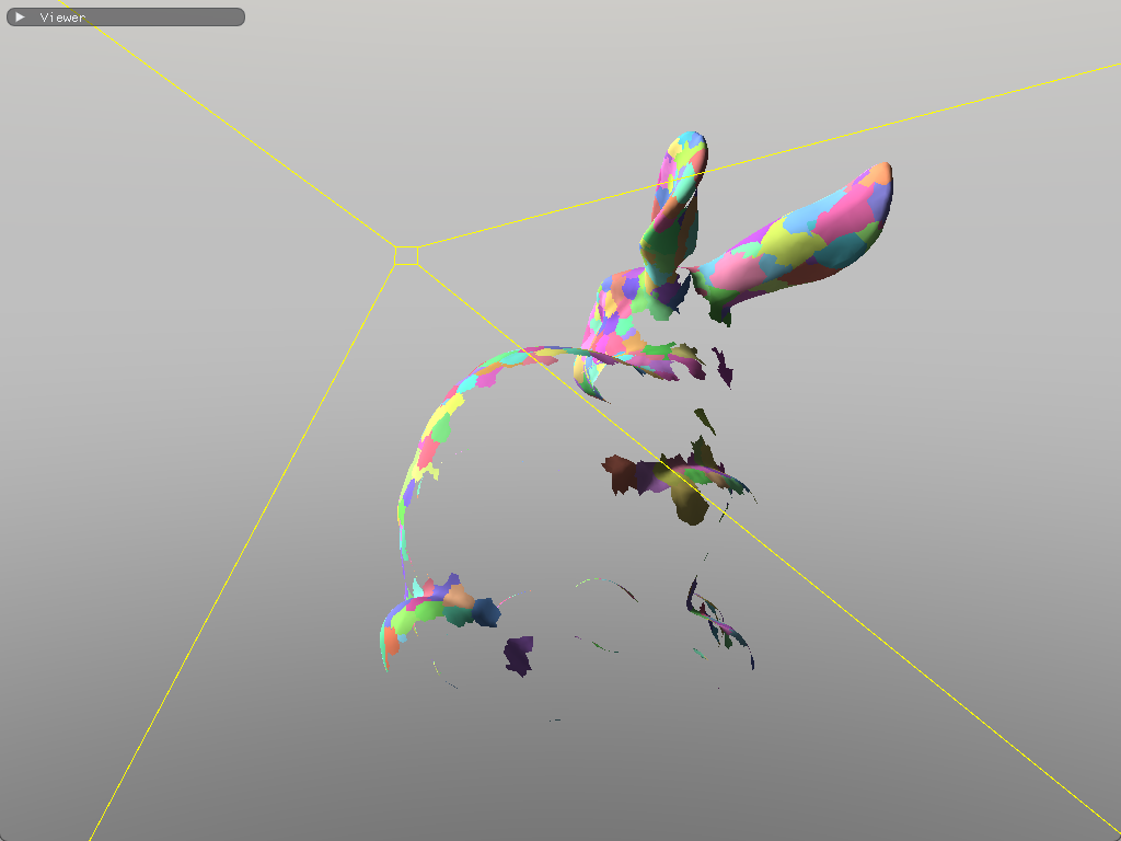
This gives us per-meshlet frustum culling. Meshlets that are outside the camera's frustum never spawn mesh shader workgroups.
Optimizing the renderer
Now that we have our task and mesh shader working, and we have control over which meshlets to dispatch, let's look for potential improvements and implement more culling methods to bring our mesh shader invocations further down.
Wave intrinsics
The pattern we're implementing in the task shader, filtering elements and compacting them into a contiguous list, is called stream compaction. However, there's a subtle inefficiency with using InterlockedAdd to achieve this.

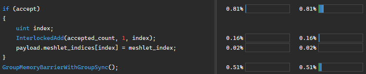
Every thread that passes the visibility test calls InterlockedAdd on the same accepted_count variable. Atomics are serialized; when multiple threads in a workgroup hit the same address simultaneously, the hardware queues them up and processes them one at a time. With 32 threads potentially contending for a single counter, we're creating a bottleneck.
Modern GPUs organize threads into groups called waves (NVIDIA) or wavefronts (AMD). Threads within a wave execute in lockstep, which enables special intrinsics that communicate between threads without explicit synchronization or atomics.
Two intrinsics are particularly useful here:
bool accept = /* all sorts of visibility tests */;
uint index = ; // returns how many threads before this one have "true"
uint count = ; // returns how many threads in the wave have "true"
if payload.meshlet_indices = meshlet_index;
If threads 0, 3, and 5 pass the visibility test, WavePrefixCountBits returns 0, 1, and 2 respectively, and WaveActiveCountBits returns 3 for all threads. Each passing thread knows exactly where to write without any atomic contention.
The full task shader becomes:
This works cleanly when the workgroup size equals the wave size (32 on NVIDIA, 32 or 64 on AMD). For larger workgroups, you'd need to handle multiple waves, using one atomic per wave to claim a range of slots rather than one per thread.
void
In this scene, we save about ~0.05ms. This was not that big of an improvement but at least we don't have atomics in our task shader anymore.
Profiling results
Backface cone culling
When we were generating our meshlets, we skipped over some fields in meshopt_Bounds:
;
For each meshlet, meshoptimizer computes a cone that bounds all triangle normals defined by an axis (cone_axis) and the cutoff angle (cone_cutoff). If the camera lies outside this cone, every triangle in the meshlet is backfacing. The function simply checks if the camera_position lies outside the cone:
Using
cone_apexcan lead to better results, although it will make backface culling more expensive to compute. In my case, backface culling seemed to perform fine without it.
bool
In the task shader, we need to transform the cone axis by the instance's rotation:
The cone data is packed efficiently. meshoptimizer provides the axis and cutoff as signed 8-bit integers, normalized to the range
[-1, 1]:
float3 cone_axis = ;
float cone_cutoff = int / 127.0;
accept = !;
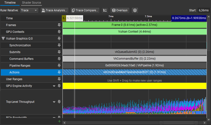
In this scene, we get about ~40% fewer mesh shader invocations from this culling technique alone:

To make meshoptimizer favor this technique, we'd have to change the cone_weight variable we mentioned earlier. The trade-off is potentially worse vertex re-use.
Occlusion culling
Frustum culling and backface culling already filter out most of our meshlets for stuff that is obviously not visible. There is one more culling technique we can implement: rejecting meshlets that are hidden behind other geometry. Hardware depth testing handles this per-pixel, but at that point we'd have already processed the vertex and assembled the primitive. We can do this much earlier into the pipeline and reject entire meshlets with Hi-Z occlusion culling.
We first grab the depth buffer and build a mipmap chain out of it. However, there is a small difference with downsampling, instead of taking the average of 4 pixels, we instead take the maximum. We dispatch a compute shader per-mip level, with the previous mip being the input:
If you check out my implementation, you will notice that I am taking the minimum instead of the maximum. This is because I am using another rendering technique called Reverse-Z which reverses depth to increase the precision of the depth buffer. For the sake of clarity, and that it's trivial to adopt Hi-Z occlusion culling with Reverse-Z, this article will not be describing occlusion culling with Reverse-Z in mind.
Sampler2D src;
RWTexture2D<float4> dst;
void
When sampling the depth pyramid, we want the hardware to return the maximum depth within the sampled region, not an interpolated value. The VK_EXT_sampler_filter_minmax extension provides this functionality through sampler reduction modes:
VkSamplerCreateInfo ;
// ...
VkSamplerReductionModeCreateInfoEXT reduction_create_info = ;
reduction_create_info.reductionMode = VK_SAMPLER_REDUCTION_MODE_MAX;
sampler_create_info.pNext = &reduction_create_info;
;
With VK_SAMPLER_REDUCTION_MODE_MAX, when we call SampleLevel, the hardware automatically returns the maximum of the sampled texels rather than a filtered blend.
The depth texture of an example scene. The resulting hierarchical depth buffer.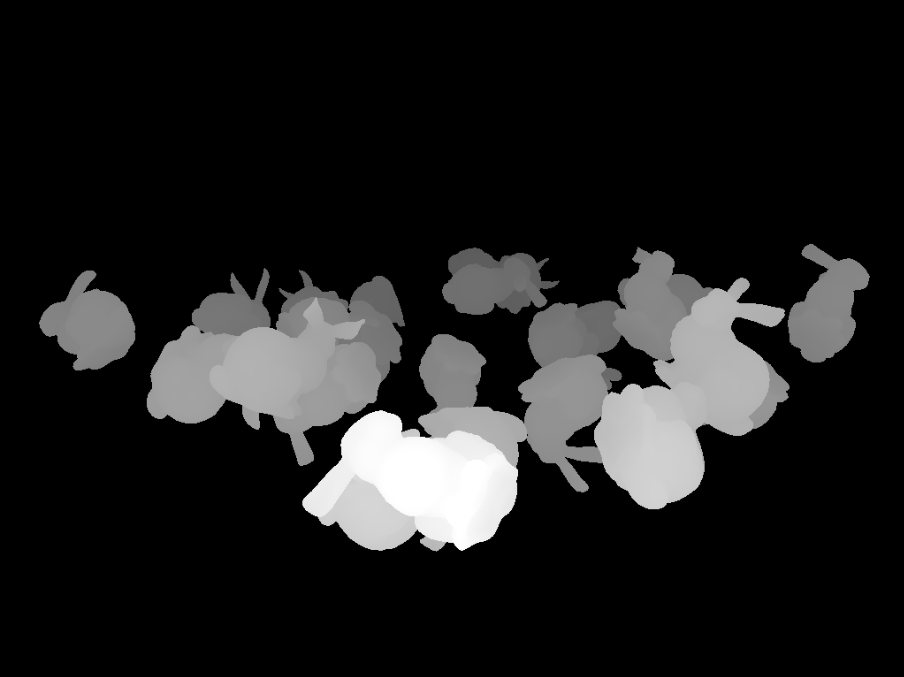
Then, for each meshlet, in the task shader, we can project its bounding sphere to screen space and get an axis-aligned bounding box.
In my implementation, I used this function to project the sphere:[12]
The function takes the sphere center in view space, not world space, so we need to transform it before calling.
bool
P00 and P11 are the projection matrix diagonal elements, projection[0][0] and projection[1][1]. With the screen-space AABB, we select the appropriate mip level based on the AABB size, sample the depth pyramid, and compare. If the nearest depth of the sphere is greater than the maximum value given by the depth chain, the object is occluded:
float4 aabb;
if

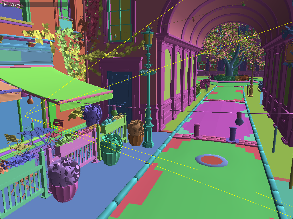
Amazon Lumberyard Bistro scene.

In my implementation, I am using the previous frame's depth. This could cause visible meshlets to be incorrectly culled for camera cuts or fast-moving objects. There are ways to mitigate this such as setting up a depth prepass, which is also used by other various rendering techniques such as SSAO and Forward+.
It is also possible to mitigate this without a depth prepass; we could rerun the culling for meshes that were discarded in the first pass, and draw any meshes that had been incorrectly culled. This is how it was implemented in Razor Engine.[13]
With meshlets and GPU culling in place, we're efficiently processing only the geometry that's actually visible. However, we're still rendering every triangle in every visible meshlet, even when those triangles are too small to meaningfully contribute to the final image.
Hierarchical LODs
Earlier we talked about the usual go-to technique for LODs in most game engines, which is having simplified meshes for each level, and based on the camera's distance to the object, a coarser mesh is picked. For big meshes, like terrain, you could split them into smaller meshlets and simplify them. However, an issue will become clear:
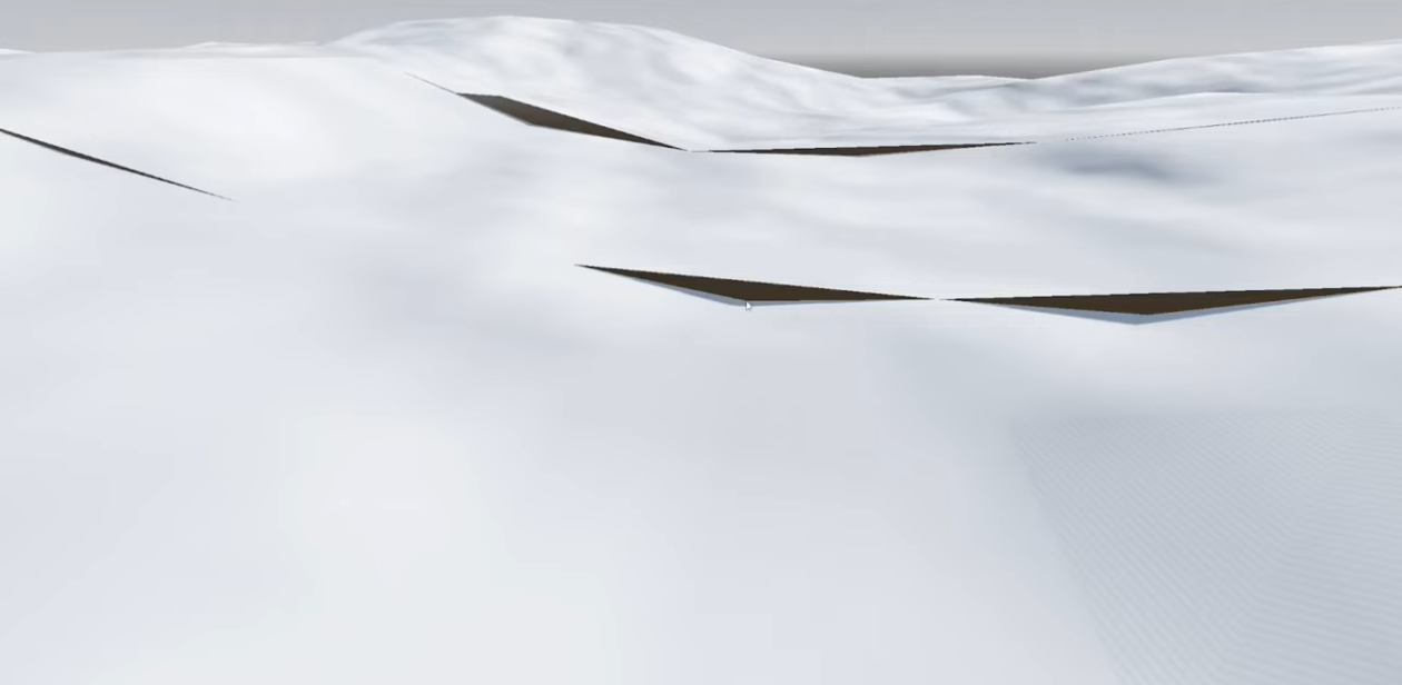
Terrain with varying LOD levels, adjacent meshes with different LOD levels picked show seams as the higher detail mesh is more subdivided, taken from this video
A naïve solution would be to preserve the boundaries of the mesh during simplification so that independent LOD levels still match. While this fixes the seam problem, it also hinders the simplification process. So much that it becomes practically impossible to even halve the triangle count per-level.
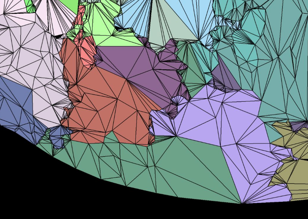
Figure taken from A Deep Dive into Nanite Virtualized Geometry
The same principles apply if we decide to generate LODs for our meshlets. We are generating smaller meshes from a bigger mesh, after all.
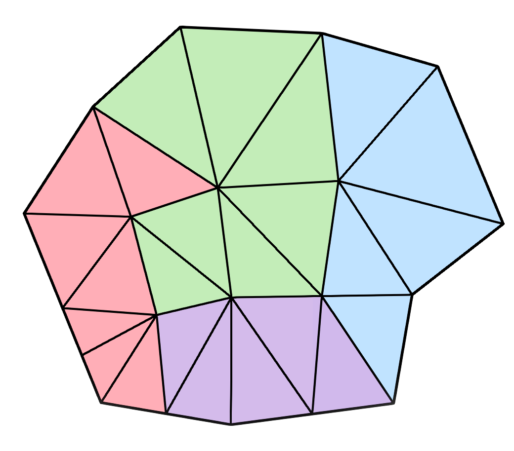
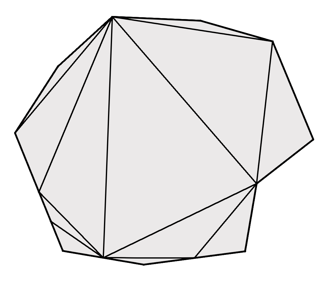
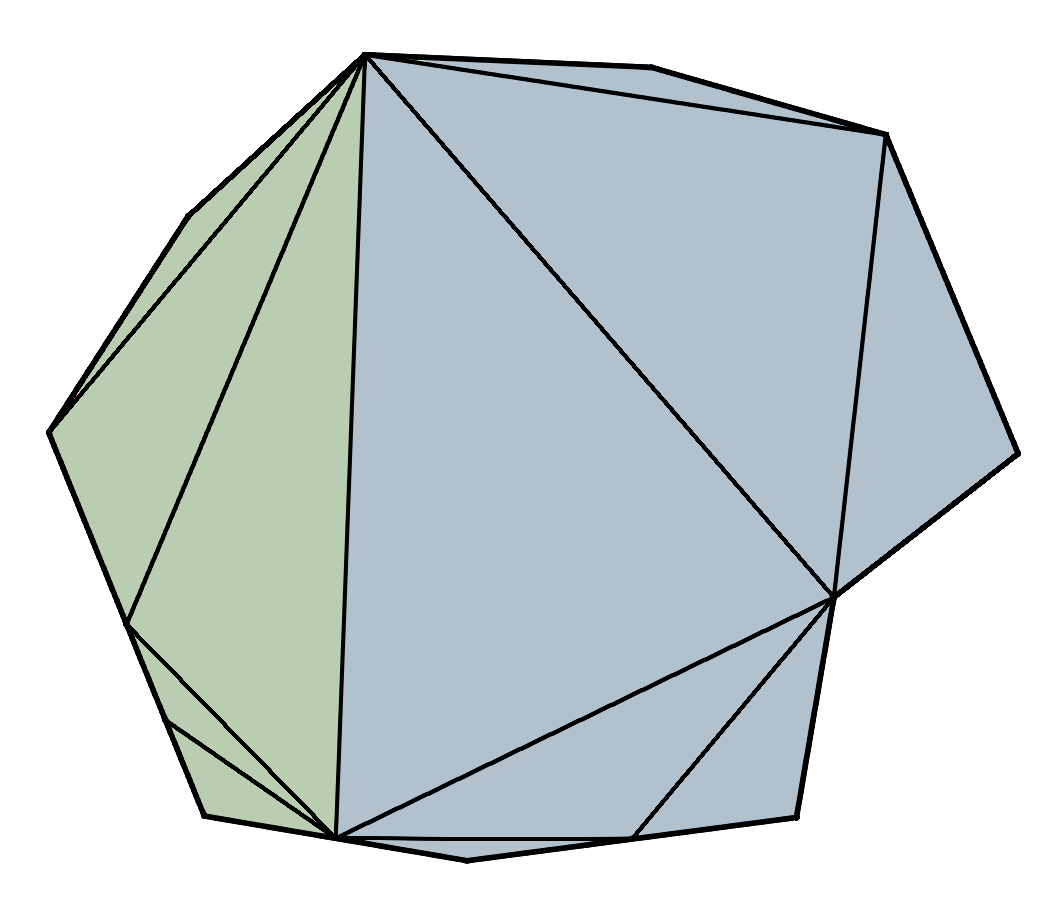
Grouping meshlets
Instead of a linear chain of LOD levels (LOD0 -> LOD1 -> LOD2 -> ...), Nanite organizes geometry into a Directed Acyclic Graph.
I know the name sounds scary, but this data structure is not that far from a tree. It is a type of graph where the edges always point in a certain direction (hence "directed"), and when walking the edges from an arbitrary starting position you will never end up at the node where you started (hence "acyclic").[14] It sounds very much like a tree but a DAG allows for multiple connections between nodes, while a tree allows for just one. So, a node can have multiple parents.

In the case of our meshes, each node in the DAG represents a group of meshlets. We begin with our original meshlets as the leaves, group adjacent meshlets together, simplify the groups by ~50%, and then split the groups back into meshlets. We repeat until we have one meshlet remaining at the root.
For my implementation, I decided to go with clusterlod.h which handles these steps very nicely by taking in the original mesh, and outputting the meshlet data, the lod hierarchy and error metrics:
;
std::vector<MeshletData> meshlets;
std::vector<LODGroupData> lod_groups;
clodConfig config = ;
config.max_vertices = 64;
;
Inside the lambda function for clodBuild we can initialize our array of lod groups:
LODGroupData ;
// Bounding sphere for the group
lod_group.center = ;
lod_group.radius = group.simplified.radius;
lod_group.error = group.simplified.error; // Maximum error introduced by simplification
lod_group.depth = group.depth; // Depth of the group in the DAG
lod_group.cluster_start = static_cast<uint32_t>;
lod_group.cluster_count = static_cast<uint32_t>;
lod_groups.;
As for the meshlets, we add the fields group_id, parent_group_id and lod_level to MeshletData so we can tell which group they belong to and the LOD level they are at:
for
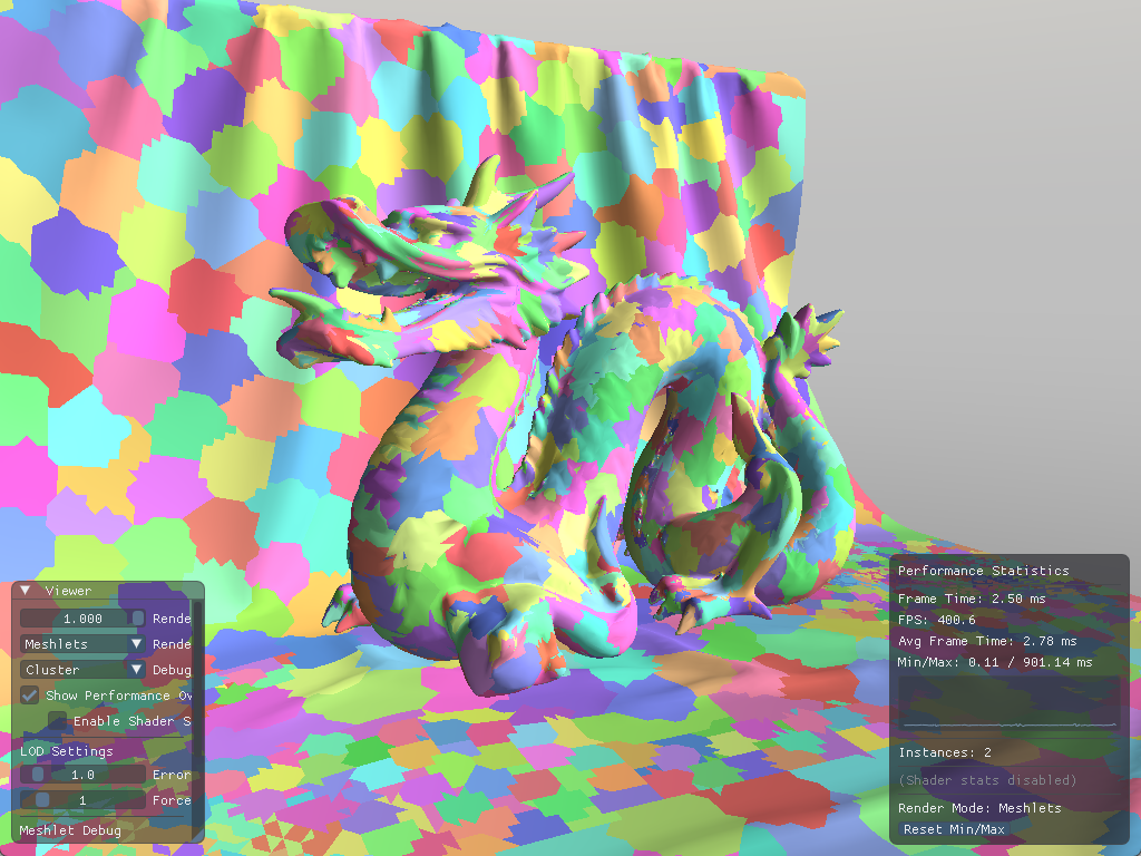
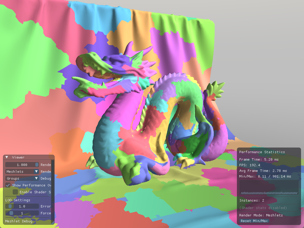
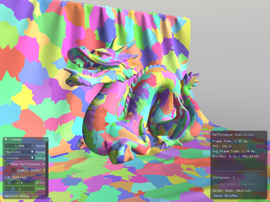
With our data ready, we can check if our LODs are generated properly by forcing an LOD level on the mesh:

The dragon mesh becomes increasingly coarser as the picked LOD level increases
Quadric Error Metric
As seen with clodBuild, our lod group struct has a field for error. This is an estimate of the error introduced by simplifying meshlets, it is an approximation of geometric deviation from the original mesh in world space.[15]
To decide whether a meshlet's error is acceptable, we project this value onto screen space:
meshoptimizer gives us the normalized error
[0..1], so we need to multiply it by screen height to get the error in pixels.
float
If the meshlet's error in pixels is below our threshold (e.g 1 pixel), the meshlets are imperceptibly different.
LOD selection
Now that our DAG and simplified meshlets are ready, and we know a bit about the error metric, let's get to picking the right LODs for each meshlet. LOD selection corresponds to cutting the DAG, it involves finding a view dependent cut of the hierarchy. However, it is simply not practical to traverse the DAG as there are many paths we can take from the root to another node, so we need to step back and consider what defines the cut.

There are two conditions that have to be met, to decide if we should render our meshlet:
- The error for the group it's in is over the error threshold.
- The parent group's error is at or under the error threshold.
The cut happens where a parent's error is too high, but its child's error is small enough to be drawn. This is great because we don't depend on which path we took to get to our meshlet, and it is perfectly suitable for parallelization, so the next step is to update our task shader with this lod selection logic:
bool
Then this function becomes our first check before culling:
bool accept = ;
accept = accept && !;
accept = accept && ;
With everything in place, we finally got ourselves a very performant renderer!
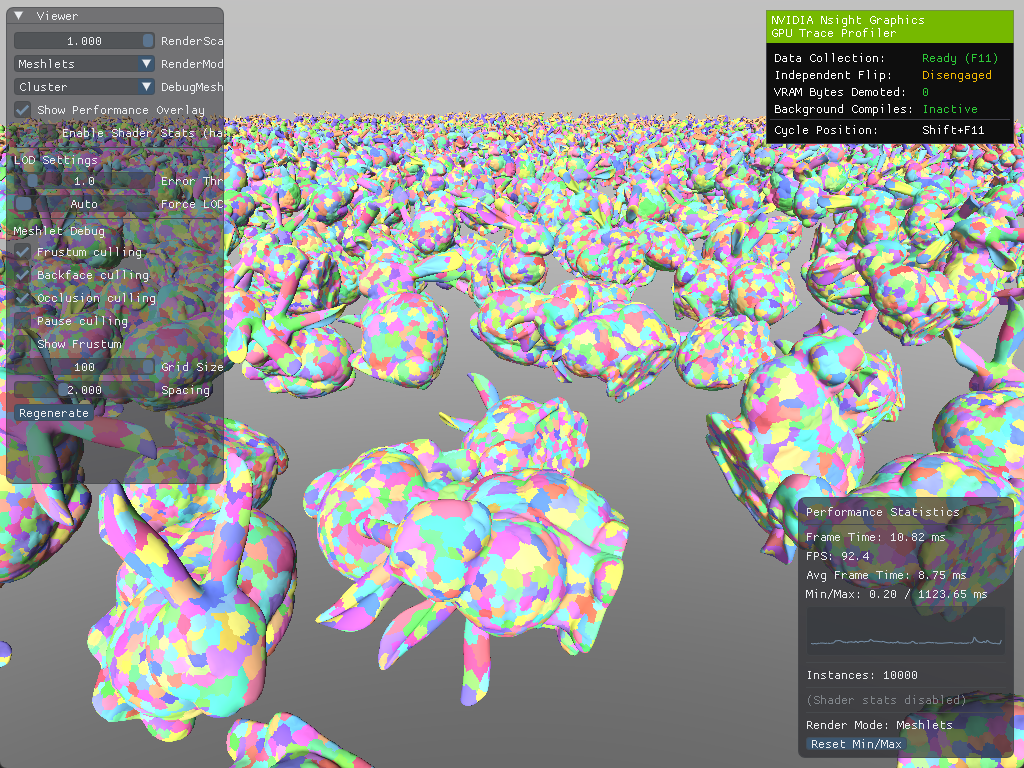
Demo
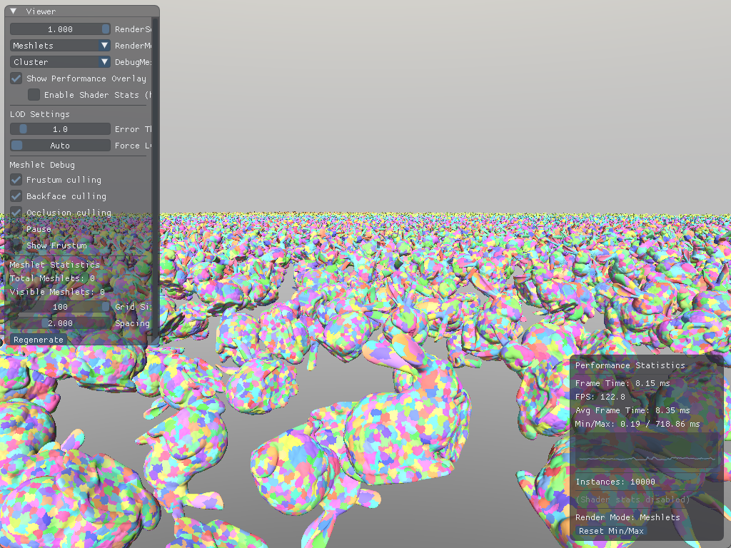
On my laptop (that's constantly thermal throttling) with an NVIDIA GeForce RTX 3080 Mobile GPU I am getting frametimes around 8-10ms to draw a scene with 10000 instances of bunnies:
You can build and try it out for yourself by cloning github.com/knnyism/Kynetic. It's licensed under MIT.
Future work
With everything that has been said, even though this article has been a gigantic one, we haven't yet implemented even half of Nanite's features. Several important features remain unexplored:
- Streaming: We don't need all the LOD data to live on the GPU at once, Nanite implements streaming to reduce VRAM usage.
- Compression: Meshlet data can be compressed significantly. Quantizing positions, using variable-length encoding for indices etc.
- Software rasterizer: For very small triangles (sub-pixel or pixel-sized), hardware rasterization becomes inefficient, Nanite addresses this with a software rasterizer that processes tiny triangles directly in compute shaders. They report it is 3x faster than hardware on average.
- Shadows: Extending this to shadow maps requires additional culling passes per shadow cascade, potentially with different error thresholds since shadow maps are often lower resolution.
Additionally:
- Skinned meshes: Extending meshlets to support skeletal animation introduces several challenges. View frustum and backface culling on a per-meshlet basis for skinned, animated models are difficult to achieve while respecting the conservative spatio-temporal bounds that are required for robust rendering results.[16]
Further reading
- Mesh and task shaders intro and basics
- Introduction to Turing Mesh Shaders
- Mastering Graphics Programming with Vulkan - repository
- A Deep Dive into Nanite Virtualized Geometry - recording
- Billions of triangles in minutes
- Virtual Geometry in Bevy 0.14
- Meshlets and Mesh Shaders
- Meshlet Rendering using DX12 Mesh Shading pipeline
- Experiments in GPU-based occlusion culling
- Creating a Directed Acyclic Graph from a Mesh
References
- [1], [9], [10] Kubisch, C. (2023, August 2). Introduction to Turing Mesh shaders. NVIDIA Technical Blog. https://developer.nvidia.com/blog/introduction-turing-mesh-shaders/
- [2] A fellow artist at BUas.
- [3] Karis, B., Stuber, R., & Wihlidal, G. (2021). A deep dive into Nanite virtualized geometry [Conference presentation]. SIGGRAPH 2021. https://advances.realtimerendering.com/s2021/Karis_Nanite_SIGGRAPH_Advances_2021_final.pdf
- [4] Chajdas, M. G. (2016, February 14). Storing vertex data: To interleave or not to interleave? Anteru's Blog. https://anteru.net/blog/2016/storing-vertex-data-to-interleave-or-not-to-interleave/
- [5] Gribb, G., & Hartmann, K. (2001, June 15). Fast extraction of viewing frustum planes from the world-view-projection matrix. GameDevs.org. https://www.gamedevs.org/uploads/fast-extraction-viewing-frustum-planes-from-world-view-projection-matrix.pdf
- [6] Wloka, M. (2003, March). "Batch, Batch, Batch:" What does it really mean? [Conference presentation]. Game Developers Conference, San Jose, CA, United States. https://www.nvidia.de/docs/IO/8230/BatchBatchBatch.pdf
- [7] Blanco, V. (n.d.). Draw indirect. Vulkan Guide. Retrieved January 11, 2026, from https://vkguide.dev/docs/gpudriven/draw_indirect/
- [8] Oberberger, M., Kuth, B., & Meyer, Q. (2023, December 19). From vertex shader to mesh shader. AMD GPUOpen. https://gpuopen.com/learn/mesh_shaders/mesh_shaders-from_vertex_shader_to_mesh_shader/
- [11] Oberberger, M., Kuth, B., & Meyer, Q. (2024, January 16). Optimization and best practices. AMD GPUOpen. https://gpuopen.com/learn/mesh_shaders/mesh_shaders-optimization_and_best_practices/
- [12] Castaño, I. (2012). "2D Polyhedral Bounds of a Clipped, Perspective-Projected 3D Sphere." Journal of Computer Graphics Techniques, 2(2), 70–83. https://jcgt.org/published/0002/02/05/
- [13] Castagno, M., & Ciardi, G. (2023). Mastering Graphics Programming with Vulkan. Packt Publishing. https://www.packtpub.com/en-us/product/mastering-graphics-programming-with-vulkan-9781803244792
- [14] Hesp, S. (2023, December 22). Creating a directed acyclic graph from a mesh. Traverse Research. https://blog.traverseresearch.nl/creating-a-directed-acyclic-graph-from-a-mesh-1329e57286e5
- [15] Garland, M., & Heckbert, P. S. (1997). Surface simplification using quadric error metrics. Proceedings of the 24th Annual Conference on Computer Graphics and Interactive Techniques (SIGGRAPH '97), 209–216. https://www.cs.cmu.edu/~garland/Papers/quadrics.pdf
- [16] Unterguggenberger, J., Kerbl, B., Pernsteiner, J., & Wimmer, M. (2021). Conservative meshlet bounds for robust culling of skinned meshes. Computer Graphics Forum, 40(7), 57–69. https://doi.org/10.1111/cgf.14401
This article and project was part of my research project at BUas 🧡